Predicting the Average Salary of an NBA Player over Their Career
- Andrew Giocondi
- Mar 12, 2022
- 9 min read

Updated: Mar 15, 2022

Introduction
Out of the existing professional sports leagues, the NBA is the highest-paying league in the world. The contracts that the players are signing continue to increase in the amount that is being made. In the 2014-2015 season the average salary was $4.45 million, while in the 2021-2022 season it is expected to be at around $8.25 million. The median salaries for these two seasons are $2.67 million and $4.02 million, respectively. Based on these values, it not only shows that there are players with massive contracts pulling the average salary higher, but also that the amount of money players are making is continuing to increase at very high rates. As a fan who follows the majority of news in the NBA, seeing some of the large-scale signings leaves me wondering whether a player is worth their contract. In addition, it leaves the desire to be able to predict what these salaries are given a particular player's statistics.
In this project, linear regression models will be used to predict the average salary of an NBA player over their career, based on various career averages and information regarding the player. The dataset being used contained a CSV file for player information and a CSV file for season and salary data. Together, it represents every NBA player from the 1984-1985 season to the 2017-2018 season. The data is sourced from basketball-reference.
What is Linear Regression?
Linear regression is a machine learning algorithm that falls into the category of supervised learning. It is a statistical method simply used to find relationships between given independent and continuous dependent variables. Meaning, it finds how the independent variables affect the dependent variable. In doing so, it assists in being able to predict the outcomes or values of something based on the linear relationship with certain variables. If more than one explanatory variable is used, like in this project, the process is called multiple linear regression.
The following formula will be derived from the linear regression model where y is the target variable, 𝛽 is the intercept, 𝛽n is the unknown parameter, xn is the independent variable, and ε is the error term:
y = 𝛽 + 𝛽1*x1 + 𝛽2*x2 + … + ε
Implementing the least-squares method, in order to find the line of best fit to represent the linear relationships, the sum of squared errors (SSE) is used. By summing the difference between the actual and predicted values which are the residuals, and then squaring them, it is able to find the best fit to minimize the errors.

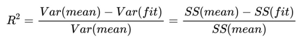
When the linear model is articulated, there are a few ways to measure its accuracy. The Coefficient of Determination (R^2) is one example, which represents how much variation in the target variable (y) can be explained by the features (x). It basically measures the goodness of fit of the model with a value of 1 being perfect and a value of 0 being the lowest.
Other examples to measure accuracy are the Mean Square Error (MSE) and the Root Mean Square Error (RMSE). Basically, the RMSE and MSE tell you how close a regression line is to a set of points. The MSE is the variance of the residuals while the RMSE is the standard deviation of the residuals.

Pre-processing and Data Understanding
Due to the reason that the data was retrieved in two separate CSV files, the first step was to merge them together based on player name and id. After doing so, the columns that seemed to be unnecessary or irrelevant in predicting an NBA player’s salary were dropped. After, there were two columns that contained null values: draft pick and draft year. I examined these variables and realized that the null values meant undrafted, therefore, I replaced them with 0’s.
The following series of preprocessing steps included row manipulation. There were many columns with data types of strings or objects that had to be changed to an integer or float format. First, the draft pick was altered into integer types. Then, the position was changed to either a 1, 2, 3, 4, or 5 to denote PG, SG, SF, PF, and C. Only the primary positions of players were kept in this case. Weight and height were also edited into integer values. In the column representing the player’s shooting hand, right-handed shooters were now 1’s, and left-handed shooters were now 0’s. Only the player’s primary shooting hand was also kept in this case. In the career FG percentage, career 3-point FG percentage, and career FT percentage columns, there existed “-” symbols to constitute no made shots. All of these instances were changed to 0’s. In the player efficiency rating (PER) and effective field goal percentage (eFG%) columns, the “-” symbols were invalid ratings, so these rows were dropped.
Afterward, a variety of graphs were made to better understand the data. The first plotted year against salaries separated into each player position.
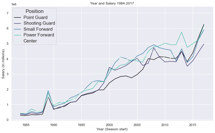
This graph portrays every season for every player rather than their career average. Due to most of the player statistics being averages over their entire career, this needed to also be reflected on the salaries and year. The dataset was grouped by player name, the mean for each column was taken, and the next graph was plotted.
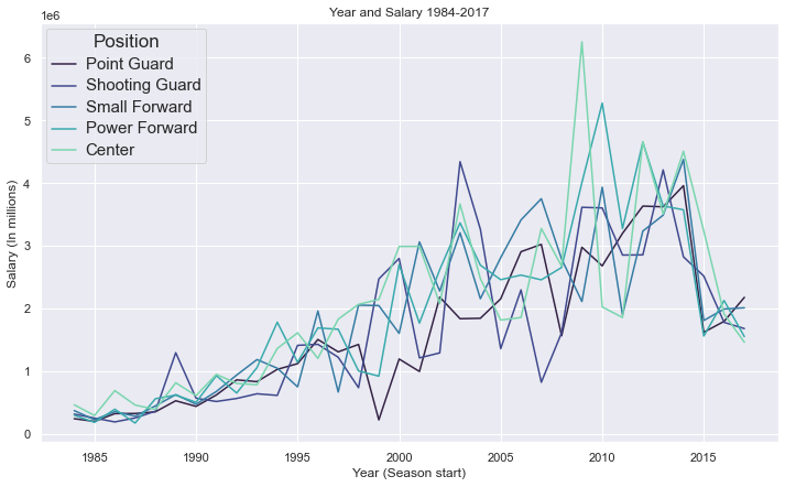
From these two graphs, it is obvious that the salary of players continues to rise. It is also apparent that the position of a player does not pose any significant difference in how much he makes over the course of every included year. An interesting aspect that can be noticed in both of these graphs is the drop in salary in the year 2014, which is the result of a decrease in salary cap for that year. In regards to the second graph that displays career salary averages, the salary is lower because players with an average playing year of 2015, 2016, and 2017 are new and have not had much time to build up their salaries.
The next series of graphs are scatter plots to show the relationships between potential independent variables and career average player salary.

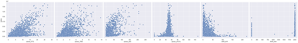

Out of these visualizations, we can view that assists, FT percentage, games played, points, rebounds, win shares, draft year, shooting hand, and season year have positive relationship with salary. Another important note is that FG percentage, 3-point FG percentage, PER, eFG%, weight, and height seem to have a range of values that are optimal for high salaries, most likely due to outliers.
Following these graphs, in order to express the correlation coefficient for the variables, the categorical variables were made into dummy variables. For these, k-1 variables were used for the analysis to treat the missing dummy variable as a baseline with which to compare all others. The dummy variables for position excluded centers, and the shooting hand excluded left-handed shooters. Furthermore, because draft pick and draft year contained 0 for undrafted players, they were made into categorical bins and dummy variables to prevent invalidation. The bins were draft pick were '1-15', '16-30', '31-45', '46-60', '>60', with undrafted being the excluded dummy variable. The bins for the draft year were '<1970', '1970-1979', '1980-1989', '1990-1999', '2000-2009', '2010-2017', with undrafted also being the excluded dummy variable.
Now, with the correlation coefficients having the ability to be calculated, a heatmap with these values was created and the relationships between all variables can be further evaluated.

Linear Regression: Experiment 1
Moving on to the modeling phase of the project, the first experiment will be the inclusion of all variables without any additional data manipulation steps. This will set a base level for our other models and make room for progress.
The following are the results (see code for more detail on how these were found):
R^2 score: 0.7213273881003481
Coefficients:
career_AST: 2.103803e+05
career_FG%: -1.117201e+04
career_FG3%: -2.313265e+03
career_FT%: -1.260122e+03
career_G: 1.013574e+03
career_PER: 1.343270e+04
career_PTS: 1.469282e+05
career_TRB: 1.041047e+05
career_WS: 1.706464e+04
career_eFG%: -3.864607e+03
weight: 5.321724e+03
height: 5.683330e+04
season_start: 4.537896e+04
PG: 5.108777e+04
SG: 1.290947e+05
SF: 3.037644e+03
PF: -1.051090e+05
Right: 4.820390e+04
1-15: -7.177568e+04
16-30: -7.138414e+05
31-45: -7.084905e+05
46-60: -8.043538e+05
>60: 3.495605e+05
<1970: -2.733615e+06
1970-1979: -2.276492e+06
1980-1989: -5.332741e+05
1990-1999: 1.142264e+06
2000-2009: 1.385190e+06
2010-2017: 1.067026e+06
Intercept: -96460236.23
Mean squared error: 1976949877732.82
Root Mean squared error: 1406040.50
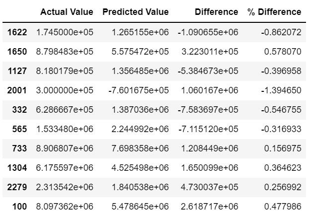
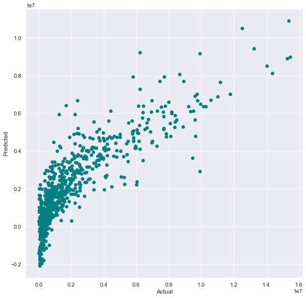
From this output, it can be concluded that the model performed fairly well for not implementing any optimization strategies. With a coefficient of determination of around 0.721, approximately 72.1% of the variation in career average salary can be explained by the included variables. However, with the MSE, RMSE, and percent difference between the actual value and predicted values being fairly large, there is definitely room for improvement. The graph below shows how well the model predicted the values in comparison to the actual values.
Linear Regression: Experiment 2
In this model, in hopes of improvement, the data was standardized and variables with high collinearity and low correlation with salary were removed. Standardizing the independent variables will allow for more consistency and the same data format. This, of course, excluded the dummy variables because they are categorical. After the standardization was completed, the dummy variables were merged back into the data. Before removing any variables, a model was created and the score below was found.
R^2 score: 0.7213273881003481
There was basically no improvement after only standardizing the data. Now, for the variable removal, FG% and eFG% were removed while PER was kept to measure a player’s offense and shooting ability. Games played was removed while win shares was kept due to high collinearity. For the measure of size, height was removed, however, weight was kept since it is correlated with salary more. All position dummy variables and both shooting hand dummy variables were removed as they seem very uncorrelated with salary. Lastly, draft pick dummy variable ‘16-30’ and draft year dummy variable ‘<1970’ were removed because they have very low correlations with salary.
The following are the results (see code for more detail on how these were found):
R^2 score: 0.724166241375694
Coefficients:
career_AST: 2.962063e+05
career_FG3%: -2.457031e+04
career_FT%: 1.037725e+04
career_PER: -4.272841e+04
career_PTS: 7.300659e+05
career_TRB: 2.829968e+05
career_WS: 7.303123e+05
weight: 2.231830e+05
season_start: 5.300917e+05
1-15: 6.279750e+05
31-45: -8.071460e+04
46-60: -1.987655e+05
>60: 8.633958e+05
1970-1979: -2.476669e+06
1980-1989: -8.600684e+05
1990-1999: 7.078168e+05
2000-2009: 8.560158e+05
2010-2017: 3.635053e+0
Intercept: 1705236.14
Mean squared error: 1956810580234.70
Root Mean squared error: 1398860.46
These results show modest advancement in the model performance. This model predicted career average salaries slightly more accurately than the first, as shown by the coefficient of determination. Approximately 72.4% of the variation in career average salary can be explained by the included variables. The MSE and RMSE are still fairly large after only a small decrease from the results in the first model.
Linear Regression: Experiment 3
This linear regression model will be tried after normalizing the data and assuring normal distribution. Multivariate normality is one of the assumptions for linear regression, so taking into account the distributions should improve the model significantly. Firstly, the data was normalized to a scale between 0 and 1. This will keep the data organized, improve its consistency, and make the transformations that are required to reach normal distribution easy to execute. Again, only the continuous variables were normalized, therefore, the dummy variables were merged back into the data after.
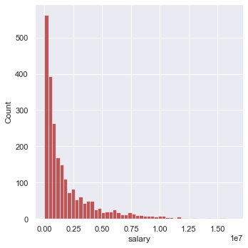
To check for normal distribution, every variable was plotted against its count. An example of this is seen below with salary.
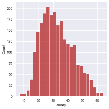
Based on how skewed the data was, square root transformations were applied for certain variables and at different strengths. Two square roots were used on assists and salary, one was used on 3-point FG percentage, points, and total rebounds, and four were used on win shares. The variables were then plotted again to display a closer level to normal distribution.
The following are the results (see code for more detail on how these were found):
R^2 score: 0.8261770185407995
Coefficients:
career_AST: 4.8377371
career_FG3%: 0.173358
career_FT%: 1.466091
career_PER: -11.153801
career_PTS: 13.278372
career_TRB: 5.967741
career_WS: 62.252423
weight: 7.768299
season_start: 9.578449
1-15: 2.572546
31-45: -2.060417
46-60: -2.378971
>60: -0.407318
1970-1979: -7.574665
1980-1989: -1.232741
1990-1999: 5.631678
2000-2009: 6.017279
2010-2017: 4.515440
Intercept: -36.52
Mean squared error: 20.45
Root Mean squared error: 4.52

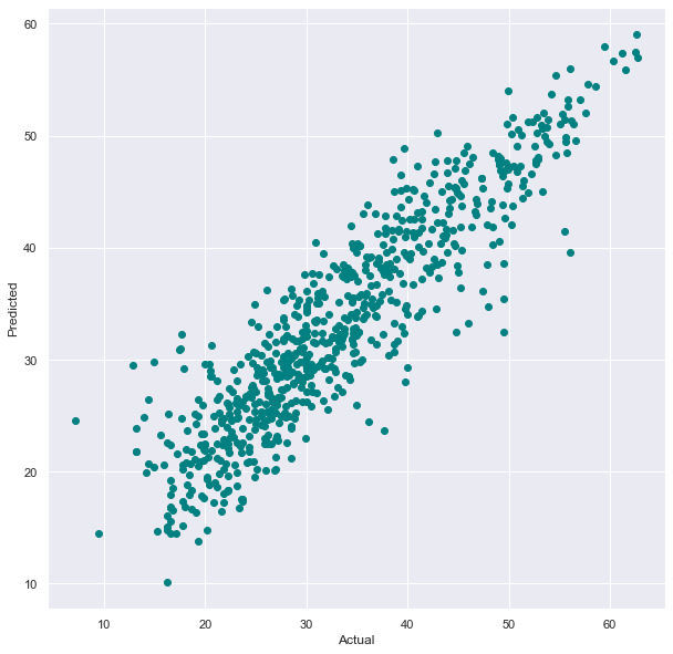
The output for this model is clearly the best one in relation to the previous experiments. The model’s performance is relatively high. With a coefficient of determination of around 0.826, approximately 82.6% of the variation in career average salary can be explained by the incorporated variables. The MSE and RMSE are quite low compared to the new scaling of the data, revealing that the regression line developed by the model fits very well in regards to the actual data. The percent difference is also low, supporting the same conclusion. Additionally, the graph below is significantly better than the graph of our first model. There are very few outliers, which proves the model's accuracy.
Ridge Regression: An Additional Experiment
To try a different type of linear regression model, the same data as used in experiment 3 will be used in ridge regression. Ridge regression is commonly used in multiple regression where the independent variables have collinearity. Even though many of the variables that had high collinearity were removed, the remaining variables still have some. The model was created and yielded the following score, which was very similar to the model output in the previous linear model:
R^2 score: 0.8261770185407995
The remaining components of the regression analysis were left out due to similarity with experiment 3. However, they can all be viewed in the code!
Conclusion
Throughout the entire process taken in this project, it was identifiable that certain steps are crucial for building a precise linear regression model. Being able to transform the data to an extent that normal distribution is met for if not all, then at least most of the variables, was the largest factor in improving model performance. Checking for collinearity, redundancy, and irrelevant variables also seemed to improve the model. Overall, I was able to gain a lot of helpful experience due to the vast amount of data in the datasets that were first retrieved as well as the lengthy amount of pre-processing steps that needed to be taken to achieve an accurate linear regression model.
I was successfully able to create a linear regression model that takes into consideration many statistics and various pieces of information regarding an NBA player’s career and predict the career average salary for that player. The model was comprised of career assists, career 3-point percentage, career free throw percentage, career player efficiency rating, career points, career total rebounds, career win shares, weight, season start year, draft pick dummy variables 1-15, 31-45, 46-60, >60, and draft year dummy variables 1970-1979, 1980-1989, 1990-1999, 2000-2009, and 2010-2017. Although there were not any specific defensive statistics, player efficiency rating and win shares directly and indirectly take into account defensive skill. Therefore, this model measures when a player was drafted, when a player played in the NBA, how well they played in the NBA, and how big they were. Together, it makes up a well-rounded description of a player for salary prediction.
Code and References
The code for this project:
The following resources were used in the process of this project.
https://www.basketball-reference.com/about/glossary.html#:~:text=Block%20percentage%20is%20an%20estimate,he%20was%20on%20the%20floor.
Cover image:


Comments